Examples
Fitting distance metric learning algorithms
>>> import numpy as np
>>> from sklearn.datasets import load_iris

>>> # Loading DML Algorithm
>>> from dml import NCA

>>> # Loading dataset
>>> iris = load_iris()
>>> X = iris['data']
>>> y = iris['target']

>>> # DML construction
>>> nca = NCA()

>>> # Fitting algorithm
>>> nca.fit(X,y)

>>> # We can look at the algorithm metadata after fitting it
>>> meta = nca.metadata()
>>> meta
{'final_expectance': 0.95771240234375,
 'initial_expectance': 0.8380491129557291,
 'num_iters': 3}

>>> # We can see the metric the algorithm has learned.
>>> # This metric is the PSD matrix that defines how the distance is measured:
>>> # d(x,y) = (x-y).T.dot(M).dot(x-y)
>>> M = nca.metric()
>>> M
array([[ 1.19098678,  0.51293714, -2.15818151, -2.01464351],
       [ 0.51293714,  1.58128238, -2.14573777, -2.10714773],
       [-2.15818151, -2.14573777,  6.46881853,  5.86280474],
       [-2.01464351, -2.10714773,  5.86280474,  6.83271473]])

>>> # Equivalently, we can see the learned linear map.
>>> # The distance coincides with the euclidean distance after applying the linear map.
>>> L = nca.transformer()
>>> L
array([[ 0.77961001, -0.01911998, -0.35862791, -0.23992861],
       [-0.04442949,  1.00747788, -0.29936559, -0.25812144],
       [-0.60744415, -0.57288453,  2.16095076,  1.35212555],
       [-0.46068713, -0.48755353,  1.25732916,  2.20913531]])

>>> # Finally, we can obtain the transformed data ...
>>> Lx = nca.transform()
>>> Lx[:5,:]
array([[ 3.35902632,  2.8288461 , -1.80730485, -1.85385382],
       [ 3.21266431,  2.33399305, -1.39937375, -1.51793964],
       [ 3.0887811 ,  2.57431109, -1.60855691, -1.64904583],
       [ 2.94100652,  2.41813313, -1.05833389, -1.30275593],
       [ 3.27915332,  2.93403684, -1.80384889, -1.85654046]])

>>> # ... or transform new data.
>>> X_ = np.array([[1.0,0.0,0.0,0.0],[1.0,1.0,0.0,0.0],[1.0,1.0,1.0,0.0]])
>>> Lx_ = nca.transform(X_)
>>> Lx_
array([[ 0.77961001, -0.04442949, -0.60744415, -0.46068713],
       [ 0.76049003,  0.9630484 , -1.18032868, -0.94824066],
       [ 0.40186212,  0.66368281,  0.98062208,  0.3090885 ]])
Similarity learning classifier extensions for Scikit-learn
>>> import numpy as np
>>> from sklearn.datasets import load_iris

>>> from dml import NCA, kNN, MultiDML_kNN

>>> # Loading dataset
>>> iris = load_iris()
>>> X = iris['data']
>>> y = iris['target']

>>> # Initializing transformer and predictor
>>> nca = NCA()
>>> knn = kNN(n_neighbors=7,dml_algorithm=nca)

>>> # Fitting transformer and predictor
>>> nca.fit(X,y)
>>> knn.fit(X,y)

# Now we can predict the labels for k-NN with the learned distance.
>>> knn.predict() # Also we can use predict(X_) for other datasets.
>>>               # When using the training set predictions are made
>>>               # leaving the sample to predict out.
array([ 0.,  0.,  0.,  0.,  0.,  0.,  0.,  0.,  0.,  0.,  0.,  0.,  0.,
        0.,  0.,  0.,  0.,  0.,  0.,  0.,  0.,  0.,  0.,  0.,  0.,  0.,
        0.,  0.,  0.,  0.,  0.,  0.,  0.,  0.,  0.,  0.,  0.,  0.,  0.,
        0.,  0.,  0.,  0.,  0.,  0.,  0.,  0.,  0.,  0.,  0.,  1.,  1.,
        1.,  1.,  1.,  1.,  1.,  1.,  1.,  1.,  1.,  1.,  1.,  1.,  1.,
        1.,  1.,  1.,  1.,  1.,  2.,  1.,  2.,  1.,  1.,  1.,  1.,  2.,
        1.,  1.,  1.,  1.,  1.,  2.,  1.,  1.,  1.,  1.,  1.,  1.,  1.,
        1.,  1.,  1.,  1.,  1.,  1.,  1.,  1.,  1.,  2.,  2.,  2.,  2.,
        2.,  2.,  2.,  2.,  2.,  2.,  2.,  2.,  2.,  2.,  2.,  2.,  2.,
        2.,  2.,  2.,  2.,  2.,  2.,  2.,  2.,  2.,  2.,  2.,  2.,  2.,
        2.,  2.,  2.,  2.,  2.,  2.,  2.,  2.,  2.,  2.,  2.,  2.,  2.,
        2.,  2.,  2.,  2.,  2.,  2.,  2.])

>>> knn.predict_proba()[-10:,:] # Again it can be used for other datasets.
array([[ 0.        ,  0.        ,  1.        ],
       [ 0.        ,  0.        ,  1.        ],
       [ 0.        ,  0.        ,  1.        ],
       [ 0.        ,  0.        ,  1.        ],
       [ 0.        ,  0.        ,  1.        ],
       [ 0.        ,  0.        ,  1.        ],
       [ 0.        ,  0.14285714,  0.85714286],
       [ 0.        ,  0.        ,  1.        ],
       [ 0.        ,  0.        ,  1.        ],
       [ 0.        ,  0.14285714,  0.85714286]])

>>> knn.score() # The classification score (score(X_,y_) for other datasets).
0.97333333333333338

>>> # We can also compare with the euclidean distance k-NN
>>> knn.score_orig()
0.96666666666666667

>>> # With MultiDML_kNN we can test multiple dmls. In this case, dmls are fitted automatically.
>>> lda = LDA()
>>> mknn = MultiDML_kNN(n_neighbors=7,dmls=[lda,nca])
>>> mknn.fit(X,y)

>>> # And we can predict and take scores in the same way, for every dml.
>>> # The euclidean distance will be added always in first place.
>>> mknn.score_all() # It will show [euclidean, lda, nca]
array([ 0.96666667,  0.96666667,  0.97333333])

>>> # The NCMC Classifier works like every ClassifierMixin.
>>> ncmc = NCMC_Classifier(centroids_num=2)
>>> ncmc.fit(X,y)
>>> ncmc.score(X,y)
0.95333333333333337

>>> # To learn a distance to use with NCMC Classifier, and with any other distance classifier
>>> # we can use pipelines.
>>> from sklearn.pipeline import Pipeline
>>> dml_ncmc = Pipeline([('nca',nca),('ncmc',ncmc)])
>>> dml_ncmc.fit(X,y)
>>> dml_ncmc.score(X,y)
0.97999999999999998
Plotting classifier regions induced by different distances
>>> import numpy as np
>>> from sklearn.datasets import load_iris
>>> from dml import NCA, LDA, NCMC_Classifier, classifier_plot, dml_plot, knn_plot,
>>> dml_multiplot, knn_pairplots
>>> # Loading dataset
>>> iris = load_iris()
>>> X = iris['data']
>>> y = iris['target']
>>> # Initializing transformers and predictors
>>> nca = NCA()
>>> lda = LDA()
>>> ncmc = NCMC_Classifier(centroids_num=2)
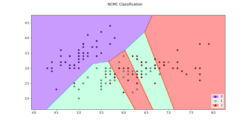
>>> # We can plot regions for different classifiers
>>> f1 = classifier_plot(X[:,[0,1]],y,clf=ncmc,title = "NCMC Classification",
>>> cmap="rainbow",figsize=(12,6))
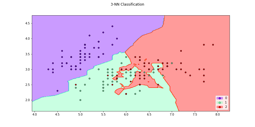
>>> f2 = knn_plot(X[:,[0,1]],y,k=3,title = "3-NN Classification", cmap="rainbow",
>>>               figsize=(12,6))
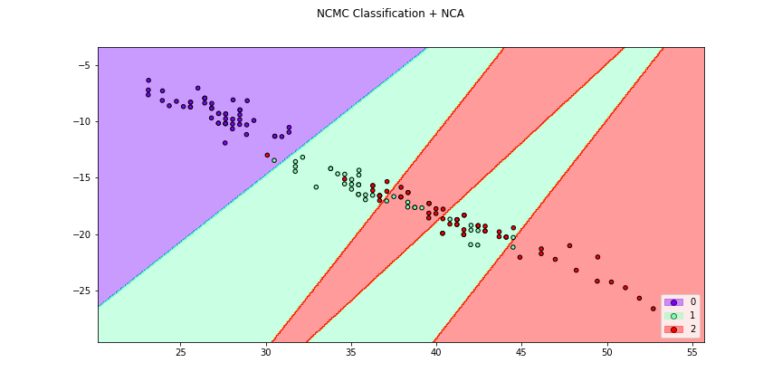
>>> # We can also make with the transformation determined by a metric,
>>> # a transformer or a DML Algorithm
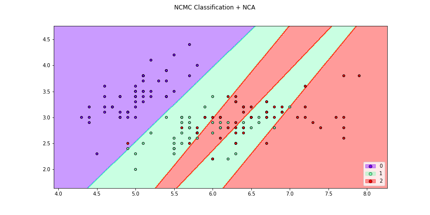
>>> f3 = dml_plot(X[:,[0,1]],y,clf=ncmc,dml=nca,title = "NCMC Classification + NCA",
>>> cmap="rainbow",figsize=(12,6))
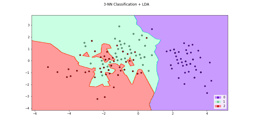
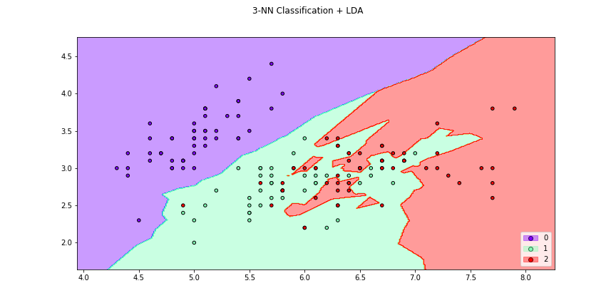
>>> f4 = knn_plot(X[:,[0,1]],y,k=2,dml=lda,title="3-NN Classification + LDA",
>>>               cmap="rainbow",figsize=(12,6))
>>> # Or we can see how the distance changes the classifier region
>>> # using the option transform=False
>>> f5 = dml_plot(X[:,[0,1]],y,clf=ncmc,dml=nca,title = "NCMC Classification + NCA",
>>>               cmap="rainbow",transform=False,figsize=(12,6))
>>> f6 = knn_plot(X[:,[0,1]],y,k=2,dml=lda,title="3-NN Classification + LDA",
>>>               cmap="rainbow",transform=False,figsize=(12,6))
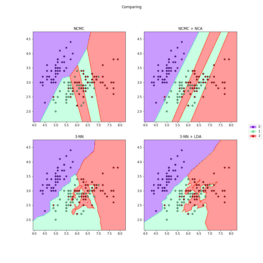
>>> # We can compare different algorithms or distances together in the same figure
>>> f7 = dml_multiplot(X[:,[0,1]],y,nrow=2,ncol=2,ks=[None,None,3,3],
>>>                    clfs=[ncmc,ncmc,None,None],dmls=[None,nca,None,lda],
>>>                    transforms=[False,False,False,False],title="Comparing",
>>>                    subtitles=["NCMC","NCMC + NCA","3-NN","3-NN + LDA"],
>>>                    cmap="rainbow",figsize=(12,12))
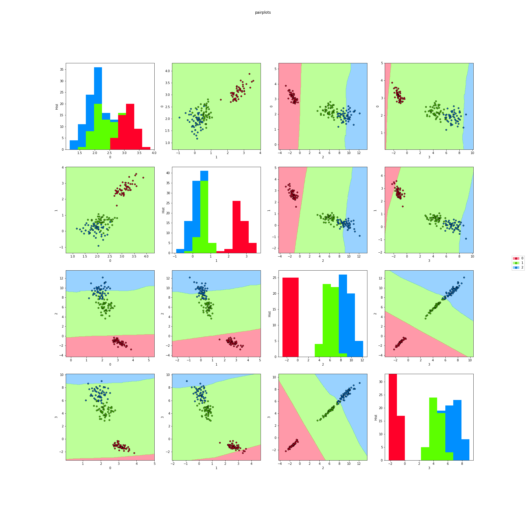
>>> # Finally, we can also plot each pair of attributes. Here the classifier region
>>> # is made taking a section in the features space.
>>> f8 = knn_pairplots(X,y,k=3,sections="mean",dml=nca,title="pairplots",
>>>                    cmap="gist_rainbow",figsize=(24,24))
Tuning parameters
>>> import numpy as np
>>> from sklearn.datasets import load_iris
>>> from dml import NCA, tune

>>> # Loading dataset
>>> iris = load_iris()
>>> X = iris['data']
>>> y = iris['target']

>>> # Using cross validation we can tune parameters for the DML algorithms.
>>> # Here, we tune the NCA algorithm, with a fixed parameter learning_rate='constant'.
>>> # The parameters we tune are num_dims and eta0.
>>> # The metrics we use are 3-NN and 5-NN scores, and the final expectance metadata of NCA.
>>> # A 5-fold cross validation is done twice, to obtain the results.
>>> results,best,nca_best,detailed = tune(NCA,X,y,dml_params={'learning_rate':'constant'},
>>>                                       tune_args={'num_dims':[3,4],'eta0':[0.001,0.01,0.1]},
>>>                                       metrics=[3,5,'final_expectance'],
>>>                                       n_folds=5,n_reps=2,seed=28,verbose=True)
*** Tuning Case  {'num_dims': 3, 'eta0': 0.001} ...
** FOLD  1
** FOLD  2
** FOLD  3
** FOLD  4
** FOLD  5
** FOLD  6
** FOLD  7
** FOLD  8
** FOLD  9
** FOLD  10
*** Tuning Case  {'num_dims': 3, 'eta0': 0.01} ...
** FOLD  1
** FOLD  2
** FOLD  3
** FOLD  4
...

>>> # Now we can compare the results obtained for each case.
>>> results
                                    3-NN      5-NN  final_expectance
{'num_dims': 3, 'eta0': 0.001}  0.963333  0.970000          0.890105
{'num_dims': 3, 'eta0': 0.01}   0.966667  0.963333          0.916240
{'num_dims': 3, 'eta0': 0.1}    0.970000  0.963333          0.935243
{'num_dims': 4, 'eta0': 0.001}  0.956667  0.963333          0.897238
{'num_dims': 4, 'eta0': 0.01}   0.956667  0.963333          0.922415
{'num_dims': 4, 'eta0': 0.1}    0.960000  0.963333          0.947319

>>> # We can also take the best result (respect to the first metric).
>>> best
({'eta0': 0.1, 'num_dims': 3}, 0.97000000000000008)

>>> # We also obtain the best DML algorithm already constructed to be used.
>>> nca_best.fit(X,y)

>>> # If we want, we can look at the detailed results of cross validation for each case.
>>> detailed["{'num_dims': 3, 'eta0': 0.01}"]
              3-NN      5-NN  final_expectance
SPLIT 1   0.966667  0.966667          0.923293
SPLIT 2   0.966667  0.966667          0.922091
SPLIT 3   1.000000  0.966667          0.907416
SPLIT 4   0.966667  0.966667          0.903700
SPLIT 5   0.966667  0.966667          0.915030
SPLIT 6   0.966667  0.966667          0.905189
SPLIT 7   0.966667  0.966667          0.922051
SPLIT 8   0.933333  0.933333          0.933400
SPLIT 9   0.966667  1.000000          0.912236
SPLIT 10  0.966667  0.933333          0.917992
MEAN      0.966667  0.963333          0.916240
STD       0.014907  0.017951          0.008888